Before we start more detailed analysis, this is the step that helps us know better about the whole data set. In this step we want to know the drug use by high school students over the United State. We are going to figure out the drug use proportion of different type of drug in each state, as well as in each race and age.

Drug use in the United States overview

The plots below show the distribution of drug use proportion in The United States.
According to CDC’s questionnaire, we define the individual who takes a drug more than 40 times as a “Heavy dose user”, the individual who takes a drug more than once and less than 40 times as a “Light dose user”, and the individual who never uses drugs as no drug user.
The plot below is the sum number of all kinds of drugs use, which contain marijuana, cocaine, inhale, heroin, ecstasy, steroid, and illegal_injection.
We can tell from the plot that the drug use proportion varies hugely among states and states. And it seems no geographical relationship between drug use proportion and states. Light drug use distribution and heavy drug use distribution do have a strong relationship.
You can find the distribution of each type of drug in this site " https://meanstudent.shinyapps.io/yrbss_overview_shinyapp/"

drug_use_overview_df = 
  drug_type_df%>%
  select(-drug_use_sum,-other_drug_sum)%>%
  pivot_longer(All_drug:illegal_injection,
               names_to = "drug_type",
               values_to = "dose")%>%
  count(state,drug_type,dose)%>%
  group_by(state,drug_type)%>%
  summarize(n,dose,sum = sum(n))%>%
  mutate(proportion = n/sum)


color_dict = hash() #Def the color of the map
color_dict[["Heavy Dose"]] = "red"
color_dict[["Light Dose"]] = "orange"
color_dict[["No Drug Use"]] = "blue"

#---------------------------------------------- Heavy Dose
Heavy_dose_df = 
    drug_use_overview_df %>%
    filter(drug_type == "All_drug",dose == "Heavy Dose")

Heavy_dose_map =   plot_usmap(data = Heavy_dose_df,values = "proportion", color = color_dict[["Heavy Dose"]],labels = TRUE) + 
  scale_fill_gradient(
    low = "white", high = color_dict[["Heavy Dose"]], name = "Proportion", label = scales::comma
  ) + theme(legend.position = "right")

Heavy_dose_map = ggplotly(Heavy_dose_map)
#---------------------------------------------- Heavy Dose



#---------------------------------------------- Light Dose
Light_dose_df = 
    drug_use_overview_df %>%
    filter(drug_type == "All_drug",dose == "Light Dose")

Light_dose_map =   plot_usmap(data = Light_dose_df,values = "proportion", color = color_dict[["Light Dose"]],labels = TRUE) + 
  scale_fill_gradient(
    low = "white", high = color_dict[["Light Dose"]], name = "Proportion", label = scales::comma
  ) + theme(legend.position = "right")
Light_dose_map = ggplotly(Light_dose_map)
#---------------------------------------------- Light Dose



#---------------------------------------------- No Drug Use
No_dose_df = 
    drug_use_overview_df %>%
    filter(drug_type == "All_drug",dose == "No Drug Use")

No_dose_map =   plot_usmap(data = No_dose_df,values = "proportion", color = color_dict[["No Drug Use"]],labels = TRUE) + 
  scale_fill_gradient(
    low = "white", high = color_dict[["No Drug Use"]], name = "Proportion", label = scales::comma
  ) + theme(legend.position = "right")

No_dose_map = ggplotly(No_dose_map)
#---------------------------------------------- No Drug Use

Heavy Drug Use Distribution

Heavy_dose_map

Light Drug Use Distribution

Light_dose_map

No Drug Use Distribution

No_dose_map

Rank of drug use

As is shown in the bar plot, AZ state has the most proportion of taking drug both in heavy dose and light dose which is 0.249789 and 0.3140928, on the contrary UT state has the least proportion of people who take drug, the proportion of students who haven’t took drug yet is: 0.7596792.

#---------------------------------------------- No Drug Use
No_drug_state_count = 
  drug_use_overview_df %>%
  filter(drug_type == "All_drug",dose == "No Drug Use")%>%
  ggplot(aes(x = fct_reorder(state,proportion,.desc = TRUE), y = proportion))+
  geom_col()+
  xlab("state")+
  coord_flip()
#---------------------------------------------- No Drug Use


#---------------------------------------------- Heavy Drug Use
Heavy_drug_state_count =
  drug_use_overview_df %>%
  filter(drug_type == "All_drug",dose == "Heavy Dose")%>%
  ggplot(aes(x = fct_reorder(state,proportion,.desc = TRUE), y = proportion))+
  geom_col()+
  xlab("state")+
  coord_flip()
#---------------------------------------------- Heavy Drug Use


#---------------------------------------------- Light Drug Use
Light_drug_state_count = 
  drug_use_overview_df %>%
  filter(drug_type == "All_drug",dose == "Light Dose")%>%
  ggplot(aes(x = fct_reorder(state,proportion,.desc = TRUE), y = proportion))+
  geom_col()+
  xlab("state")+
  coord_flip()
#---------------------------------------------- Light Drug Use

Heavy Drug Rank

ggplotly(Heavy_drug_state_count)

Light Drug Rank

ggplotly(Light_drug_state_count)

No Drug Rank

ggplotly(No_drug_state_count)

Drug type exploration

Now we have a basic intuition of drug use in the United States. Now let’s see how these eight kinds of drugs are different from others.

heavy_count = 
  drug_type_df%>%
  select(-drug_use_sum,-other_drug_sum,-sex)%>%
  mutate(race4 = as.factor(race4))%>%
  pivot_longer(All_drug:illegal_injection,
               names_to = "drug_type",
               values_to = "dose")%>%
  filter(drug_type != "All_drug")%>%
  group_by(drug_type,dose)%>%
  summarise(numbers = n())%>%
  filter(dose == "Heavy Dose")%>%
  ggplot(aes(x = fct_reorder(drug_type,numbers,.desc = TRUE),y = numbers))+
  geom_col()+
  coord_flip()+
  labs(title = "Heavy drug use")+
  xlab("")

lite_count = 
  drug_type_df%>%
  select(-drug_use_sum,-other_drug_sum,-sex)%>%
  mutate(race4 = as.factor(race4))%>%
  pivot_longer(All_drug:illegal_injection,
               names_to = "drug_type",
               values_to = "dose")%>%
  filter(drug_type != "All_drug")%>%
  group_by(drug_type,dose)%>%
  summarise(numbers = n())%>%
  filter(dose == "Light Dose")%>%
  ggplot(aes(x = fct_reorder(drug_type,numbers,.desc = TRUE),y = numbers))+
  geom_col()+
  coord_flip()+
  labs(title = "Light drug use")+
  xlab("")

Drug_use_count = heavy_count + lite_count
Drug_use_count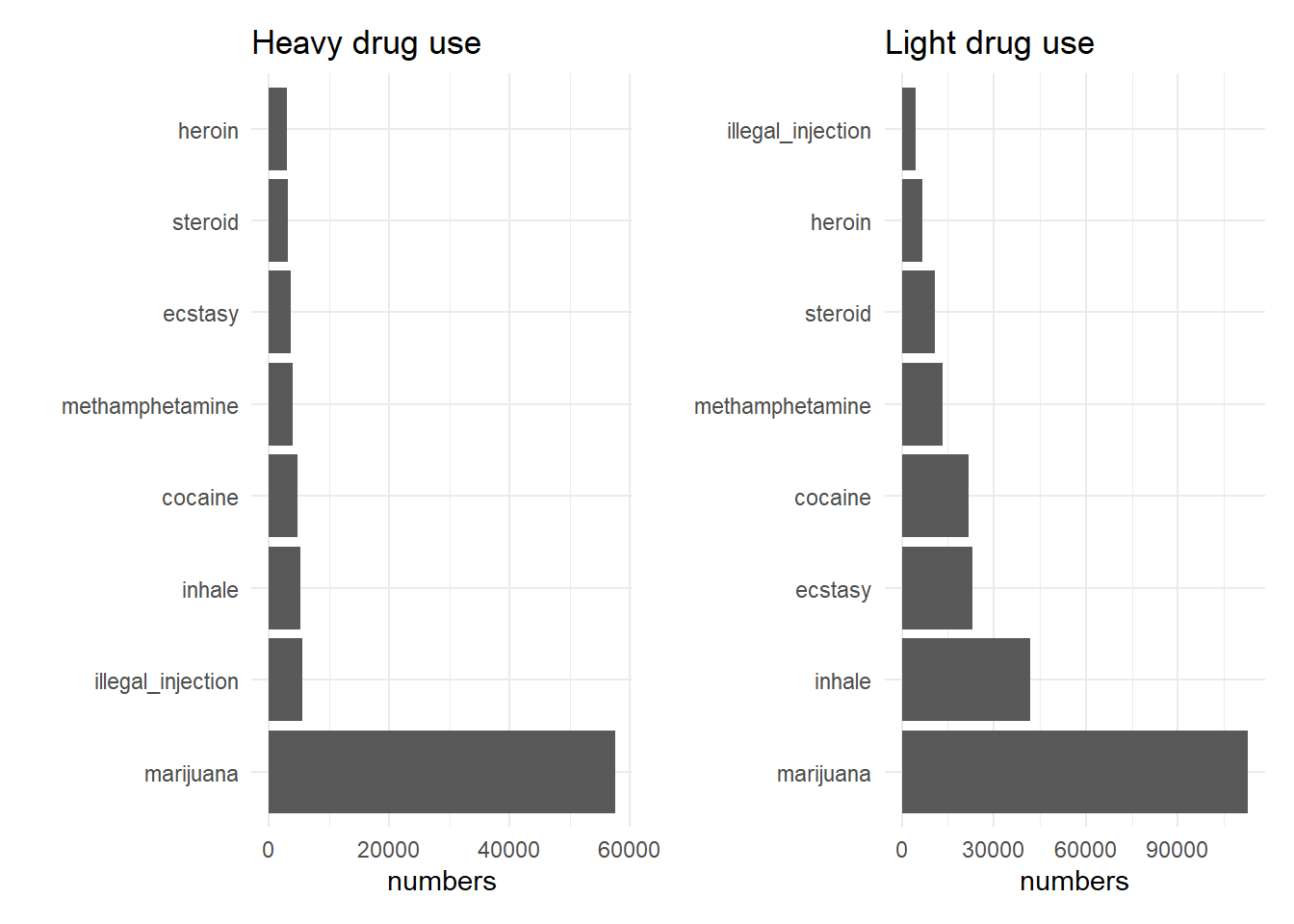

We can tell that marijuana is the most popular drug overall drugs and the number of marijuana users is even more than the sum of other drugs users.

drug_type_df%>%
  select(-drug_use_sum,-other_drug_sum,-sex)%>%
  mutate(race4 = as.factor(race4))%>%
  pivot_longer(All_drug:illegal_injection,
               names_to = "drug_type",
               values_to = "dose")%>%
  filter(drug_type != "All_drug",dose != "No Drug")%>%
  group_by(drug_type,dose)%>%
  summarise(numbers = n())%>%
  filter(dose != "No Drug Use")%>%
  pivot_wider(drug_type:dose,names_from = dose,values_from = numbers)%>%
  janitor::clean_names()%>%
  mutate(ratio = heavy_dose/light_dose)%>%
  ggplot(aes(x = fct_reorder(drug_type,ratio),y = ratio))+
  geom_col()+
  xlab("Drug type")+
  ggtitle("Heavy dose/Light Dose")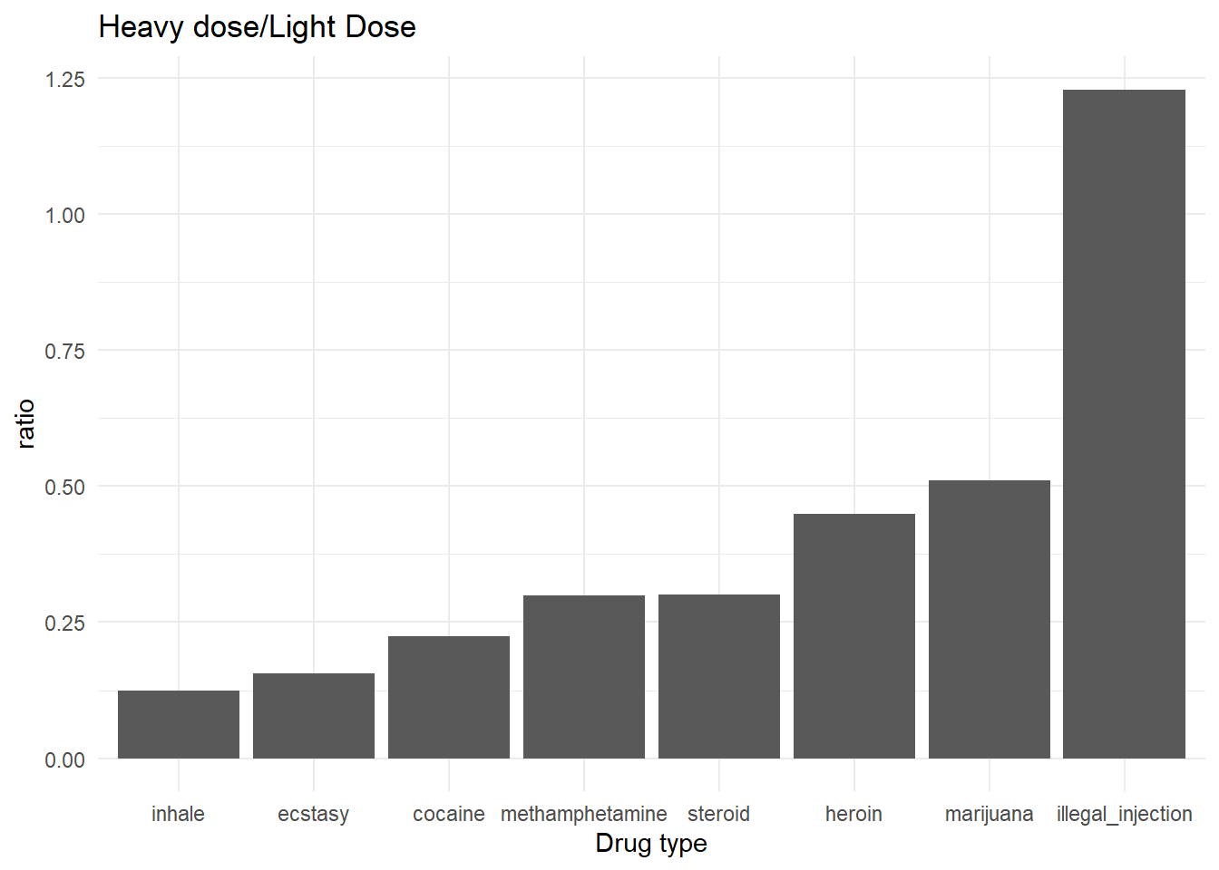

Still, we can find other useful information. The plot above is the ratio of heavy drug users and light drug users of each type of drug. A drug type with a higher ratio value means the individual who takes this drug is more likely to transfer into a heavy drug user.
This ratio does not simply stand for addiction. Other properties like properties drugs’ price, rarity… also can influence the ratio.

Drug proportion in each states.

First, we find the Top 3 most commonly used drugs, which are marijuana, inhale and ecstasy and see their difference in each state and race.
Again you can see the plot of all drugs in the following. site:“https://meanstudent.shinyapps.io/yrbss_overview_shinyapp/”

drug_type_df%>%
  select(-drug_use_sum,-other_drug_sum,-sex)%>%
  mutate(race4 = as.factor(race4))%>%
  pivot_longer(All_drug:illegal_injection,
               names_to = "drug_type",
               values_to = "dose")%>%
  filter(drug_type != "All_drug",dose != "No Drug")%>%
  group_by(drug_type,dose)%>%
  summarise(numbers = n())%>%
  filter(dose != "No Drug Use")%>%
  pivot_wider(drug_type:dose,names_from = dose,values_from = numbers)%>%
  janitor::clean_names()%>%
  mutate(sum = heavy_dose+light_dose)%>%
  arrange(sum)%>%
  tail(3)%>%
  knitr::kable()

drug_type	heavy_dose	light_dose	sum
ecstasy	3583	23074	26657
inhale	5209	41997	47206
marijuana	57583	112863	170446

drug_state_race_df = #Mutate the race to their names
  drug_type_df%>%
  select(-drug_use_sum,-other_drug_sum,-sex)%>%
  mutate(race4 = case_when(
    race4==1 ~ "White",
    race4==2 ~ "Black",
    race4==3 ~ "Hispanic/Latino",
    race4==4 ~ "All Other Races",
  ))%>%
  mutate(race4 = as.factor(race4))%>%
  pivot_longer(All_drug:illegal_injection,
               names_to = "drug_type",
               values_to = "dose")%>%
  count(state,race4,drug_type,dose)%>%
  group_by(state,race4,drug_type)%>%
  mutate(sum = sum(n),proportion = n/sum)%>%
  select(state,race4,drug_type,dose,proportion)
Drug_sum = drug_state_race_df%>%
    filter(drug_type == "All_drug")%>%
    ggplot(aes(x = state,y = proportion,color = dose))+
    scale_color_manual(values= c("#FF3225","#F5D247","#4728FA"))+
    geom_col()+
    facet_wrap(~race4)+
    coord_flip()
Marijuana = drug_state_race_df%>%
    filter(drug_type == "marijuana")%>%
    ggplot(aes(x = state,y = proportion,color = dose))+
    scale_color_manual(values= c("#FF3225","#F5D247","#4728FA"))+
    geom_col()+
    facet_wrap(~race4)+
    coord_flip()
Ecstasy = drug_state_race_df%>%
    filter(drug_type == "ecstasy")%>%
    ggplot(aes(x = fct_reorder(state,proportion),y = proportion,color = dose))+
    scale_color_manual(values= c("#FF3225","#F5D247","#4728FA"))+
    geom_col()+
    facet_wrap(~race4)+
    coord_flip()
Inhale = drug_state_race_df%>%
    filter(drug_type == "inhale")%>%
    ggplot(aes(x = fct_reorder(state,proportion),y = proportion,color = dose))+
    scale_color_manual(values= c("#FF3225","#F5D247","#4728FA"))+
    geom_col()+
    facet_wrap(~race4)+
    coord_flip()

From the following plots, we can tell that marijuana use in each race doesn’t have a big difference, however, white people seem to have less proportion of having ecstasy and inhaling drugs than other races.

All_drug

ggplotly(Drug_sum)

Marijuana

ggplotly(Marijuana)

Ecstasy

ggplotly(Ecstasy)

Inhale

ggplotly(Inhale)

Drug use in different age

pyramid plot below shows the proportion of drug users distributed in each age and sex. (The proportion is calculated separately for male and female).
The proportion of individuals younger than or equal to 13 is unstable, which is because the sample is too small(only 567 individuals younger than 13 and 578 individuals who are 13.), so we simply omit the individuals who are younger than 14 in the pyramid plot.
Of all the light dose drug users, females have a greater proportion than males. On the other hand, of all the heavy-dose drug users, males have a greater proportion than females. This means males have a higher chance than females to transfer into heavy-dose drug users.

drug_age_gender_df =
    drug_type_df%>%
    drop_na(age)%>% # drop 325 obs with out age
    select(sex,age,All_drug:illegal_injection)%>%
    mutate(sex = case_when(
      sex == 2 ~ "Male",
      sex == 1 ~ "Female"
    ),
           age = case_when(
      age == 1 ~ "<13",
      age == 2 ~ "13~14",
      age == 3 ~ "14~15",
      age == 4 ~ "15~16",
      age == 5 ~ "16~17",
      age == 6 ~ "17~18",
      age == 7 ~ "18+"
    ))%>%
    mutate(age = as.factor(age))%>%
    pivot_longer(All_drug:illegal_injection,
                 names_to = "drug_type",
                 values_to = "dose")%>%
    filter(drug_type == "All_drug")%>%
    group_by(sex,age,dose)%>%
    summarise(age_count = n())%>%
    group_by(sex,age)%>%
    summarise(dose,age_count,dose_count = sum(age_count))%>%
    filter(age != "<13" && age != "13~14")


#---------------------------------------------------------------Light dose pyramid
Light_drug_use_pyramid = 
  drug_age_gender_df%>%
  filter(dose == "Light Dose")%>%
  mutate(proportion = age_count/dose_count)

Light_pyramid_plot = 
  Light_drug_use_pyramid%>%
    ggplot(aes(x = age, fill = sex, y= ifelse(test = sex == "Male",
                                                  yes = -proportion, no = proportion))) +
    geom_bar(stat = "identity",aes(text = str_c("Age:",age,"\n","Gender:",sex,"\n","Proportion:",proportion))) +
    scale_y_continuous(labels = abs, limits = max(Light_drug_use_pyramid$proportion) * c(-1,1)) +
     labs(x = "Age", y = "Percent population of corresponding sex")+
    coord_flip()

Light_pyramid_plot = ggplotly(Light_pyramid_plot,tooltip = "text")
#---------------------------------------------------------------Light dose pyramid


#---------------------------------------------------------------Heavy dose pyramid
Heavy_drug_use_pyramid = 
  drug_age_gender_df%>%
  filter(dose == "Heavy Dose")%>%
  mutate(proportion = age_count/dose_count)

Heavy_pyramid_plot = 
  Heavy_drug_use_pyramid%>%
    ggplot(aes(x = age, fill = sex, y= ifelse(test = sex == "Male",
                                                  yes = -proportion, no = proportion))) +
    geom_bar(stat = "identity",aes(text = str_c("Age:",age,"\n","Gender:",sex,"\n","Proportion:",proportion))) +
    scale_y_continuous(labels = abs, limits = max(Heavy_drug_use_pyramid$proportion) * c(-1,1)) +
     labs(x = "Age", y = "Percent population of corresponding sex")+
    coord_flip()

Heavy_pyramid_plot = ggplotly(Heavy_pyramid_plot,tooltip = "text")
#---------------------------------------------------------------Heavy dose pyramid


#---------------------------------------------------------------No Drug use pyramid
No_drug_use_pyramid = 
  drug_age_gender_df%>%
  filter(dose == "No Drug Use")%>%
  mutate(proportion = age_count/dose_count)

No_drug_pyramid_plot = 
  No_drug_use_pyramid%>%
    ggplot(aes(x = age, fill = sex, y= ifelse(test = sex == "Male",
                                                  yes = -proportion, no = proportion))) +
    geom_bar(stat = "identity",aes(text = str_c("Age:",age,"\n","Gender:",sex,"\n","Proportion:",proportion))) +
    scale_y_continuous(labels = abs, limits = max(No_drug_use_pyramid$proportion) * c(-1,1)) +
     labs(x = "Age", y = "Percent population of corresponding sex")+
    coord_flip()

No_drug_pyramid_plot = ggplotly(No_drug_pyramid_plot,tooltip = "text")
#---------------------------------------------------------------No Drug use pyramid

Heavy Dose

Heavy_pyramid_plot

Light Dose

Light_pyramid_plot

No Drug Use

No_drug_pyramid_plot

Marijuana and Other Durgs Use Proportion

Marijuana is the most abused drug, we are interested in the marijuana drug use proportion, as well as all other drugs use proportion across the states. According to the plot, most of the states has the overall drug use proportion greater than 50%. We found that Arizona has the largest proportion of marijuana use among the youth, which is 52%. Arizona also has the highest other drug use proportion of 32%. We could also found in the plot that the states having high proportion of marijuana use are those in which marijuana use is legal, whereas the states which make it illegal have low rate of marijuana such as Utah, Iowa, and Nebraska.

if_use = function(input_list){
  output = case_when(input_list == 0 ~ FALSE,
                     input_list != 0 ~ TRUE)
}
state_proportion_drugtype = yrbss_state %>% 
  select(state, marijuana, cocaine, inhale, heroin, methamphetamine, ecstasy, steroid, illegal_injection) %>% 
  mutate(marijuana = if_use(marijuana),
         others = cocaine + inhale + heroin + methamphetamine + 
           ecstasy + steroid + illegal_injection,
         others = if_use(others)) %>% 
  select(state, marijuana, others) %>% 
  group_by(state) %>% 
  summarise(total_population = n(),
            marijuana = sum(marijuana),
            others = sum(others)) %>% 
  mutate(proportion_marijuana = marijuana / total_population,
         proportion_others = others / total_population,
         total_proportion = proportion_marijuana + proportion_others) %>% 
  pivot_longer(proportion_marijuana:proportion_others,
               names_to = "drug_type",
               values_to = "proportion") %>% 
  mutate(drug_type = recode(drug_type, 
                            proportion_marijuana = "marijuana",
                            proportion_others = "other drugs"))
state_age = yrbss_state %>% 
  select(state, marijuana_use_freq, age_marijuana) %>% 
  filter(marijuana_use_freq != "No Drug Use") %>% 
  group_by(state, marijuana_use_freq) %>% 
  summarise(mean_start_age = mean(age_marijuana, na.rm = TRUE))

state_bar_lower = state_proportion_drugtype %>% 
  filter(total_proportion < 0.5) %>% 
  plot_ly(x = ~state, y = ~proportion, 
          color = ~drug_type, type = "bar")

state_bar_greater = state_proportion_drugtype %>% 
  filter(total_proportion >= 0.5) %>% 
  plot_ly(x = ~state, y = ~proportion, 
          color = ~drug_type, type = "bar")

Drug Use Less Than 50%

state_bar_lower

Drug Use More Than 50%

state_bar_greater

The Average Starting Age of Marijuana

We are also interested in the average of the age that the youth first use marijuana. We tried to find if the mean starting age has a different pattern for each state. According to the plot in dashboard, although the mean starting age are relatively similar for each state, we found that Arizona still has the youngest starting age, which means that Arizona has severe problem of marijuana abuse not only for the proportion, but also for the starting age. Moreover, by comparing the plot of light dose and heavy dose, we discover that people who have heavy dose generally start to use marijuana earlier than those who have light dose.

state_age_heavy = state_age %>% 
  filter(marijuana_use_freq == "Heavy Dose")
state_age_light = state_age %>% 
  filter(marijuana_use_freq == "Light Dose")
  
map_plot_heavy = plot_usmap(data = state_age_heavy, values = "mean_start_age", color = color_dict[["Heavy Dose"]], labels = TRUE) + 
  scale_fill_gradient(
    low = "white", high = color_dict[["Heavy Dose"]], name = "Mean Marijuana Start Age", label = scales::comma
  ) + theme(legend.position = "right")

map_plot_light = plot_usmap(data = state_age_heavy, values = "mean_start_age", color = color_dict[["Light Dose"]], labels = TRUE) + 
  scale_fill_gradient(
    low = "white", high = color_dict[["Light Dose"]], name = "Mean Marijuana Start Age", label = scales::comma
  ) + theme(legend.position = "right")

Heavy Dose

ggplotly(map_plot_heavy)

Light Dose

ggplotly(map_plot_light)

Data Exploration

Drug use in the United States overview

Heavy Drug Use Distribution

Light Drug Use Distribution

No Drug Use Distribution

Rank of drug use

Heavy Drug Rank

Light Drug Rank

No Drug Rank

Drug type exploration

Drug proportion in each states.

All_drug

Marijuana

Ecstasy

Inhale

Drug use in different age

Heavy Dose

Light Dose

No Drug Use

Marijuana and Other Durgs Use Proportion

Drug Use Less Than 50%

Drug Use More Than 50%

The Average Starting Age of Marijuana

Heavy Dose

Light Dose